Solving symmetric disordered systems

In this post I want to describe a solution to a special class of symmetric disordered quantum systems. This solution is probably not new (it is pretty hard to come up with any solvable system which hasn’t been discovered before!) but I haven’t been able to find anything quite like it in a preliminary search of the literature. So I thought I’d write it up here; if anyone has seen something like this before then please let me know!

This research is intended to be part of a larger project focussed on the computational complexity of disordered quantum systems: I’m starting by collecting results on solvable models to subsequently utilise in the analysis of algorithms like the density matrix renormalisation group.

 

1. Disorder and symmetric quantum systems

The system I want to consider today is that of a single scalar particle hopping on a finite graph. Such systems arise, eg., in the study of conduction when one studies electrons moving through some regular lattice of atoms. However, as you’ll see, the model I want to talk about today doesn’t really arise in from any naturally occurring material.

Usually, when one studies the conduction of electrons one can reduce the problem, after several approximations, to understanding how a single electron hops between bound states of atoms in the lattice. Reflecting the approximation that the electron is assumed to be located in a definite orbital of atom we often approximate the electron position with a basis , where runs over all locations in the lattice. Notice that we have reduced the continuous degree of freedom of the electron to a discrete degree of freedom .

Now, since the orbitals of the atoms in the lattice are not completely localised there is some overlap between them. In a regular lattice there is usually only an appreciable overlap between the orbitals of neighbouring atoms. So there is some possibility for the electron at some lattice location to tunnel to a neighbouring location. Thus the energy of a single electron in the lattice may be approximated by

where is the potential felt by the electron at lattice site and represents a sum over all neighbouring lattice sites. The magnitude of the overlap between the neighbouring orbitals is wrapped up in the constant . Please note that this discussion is purely metaphorical and I’ve made a caricature of the actual details of the actual approximations involved in the correct derivation; I’ve swept a great deal under the carpet. Now, the first term in (1) is the hopping term, and this generates the dynamics of an initially localised electron at position . In real systems there is a lot of dirt and defects, so the potential tends to vary from site to site. In fact, one can often successfully model as a random variable. If we do this in the case of an electron hopping along a D line then we obtain the Anderson model.

When a system such as (1) is clean, i.e., not in the presence of a disordered potential, one typically finds that the eigenstates of the system are completely delocalised (they are regular eigenstates of momentum). In this case the electron can zoom through the lattice freely and the material becomes an excellent conductor; you should think of the electron not as a particle here, but as a wave, like a beam of light, propagating through some transparent medium. However, something remarkable happens when the potential is random: the electron gets scattered by the impurities in the potential. In fact, it gets scattered multiple times: it gets scattered so much that it becomes trapped — localised — at it’s initial location. This is the ubiquitous phenomenon of Anderson localisation.

Anderson localisation is a quantum phenomena: a classical argument based on the kinetic energy alone would lead you to expect that a classical particle would simply zoom over the rugged potential landscape without ever bouncing back. Actually, I should say it is a wave phenomena because, amazingly, Anderson localisation occurs in a wide variety of systems. There is a wonderful example explained by Sir Michael Berry: take a stack of overhead transparency films. This is a stack of transparent films with slightly random widths. At the boundary between the films an incident wave of light is partially reflected and transmitted. Now, this can be modelled as a 1D lattice of random scatterers — just like the Anderson model. One would therefore expect that light is localised in such a medium, i.e., it can’t propagate far into the stack. Thus the light can’t shine through the stack, and is thus reflected: a stack of OHP transparencies looks silver because all incident light is reflected thanks to Anderson localisation!

Disordered systems such as the Anderson model are extremely challenging to solve, to put it mildly. There are very many subtle mathematical problems which arise when trying to solve systems such as (1). The literature is roughly broken into two branches: the physical and the mathematical. The physical literature is far ahead of the mathematical literature at the current time, and I think it is fair to say that we have a pretty solid understanding of the physics of disordered systems such as (1). There are only a couple of controversies left in the theory for systems on regular lattices, centred on the two-dimensional case where some issues are not resolved. The physical literature makes heavy use of quantum-field theoretical methods, (which is what makes it hard to make rigourous) and the premiere tool to study disordered systems is the supersymmetric method pioneered by Efetov.

The mathematical literature is far behind the predictions obtained via physical arguments. The state of the art is summarised in this paper. Some things are known rigourously: it is understood that systems like (1) are localised for strong enough disorder. However, little, if anything, is known about systems which remain delocalised in the presence of small amounts of disorder. Additionally, it is extremely hard to say anything rigourously about observable quantities which are averaged over disorder. Even using physical arguments this is still rather challenging: the supersymmetric method is well-adapted to such questions, but it is restricted (as far as I can tell) to gaussian-distributed disorder.

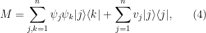
Now this discussion is meant to be a motivation of sorts for the actual system whose solution I want to describe today. This system is far from realistic, although it might arise as a mean-field limit of a strongly interacting collection of particles with long-range interactions. The system is given by

i.e., it represents a scalar particle which can hop between any of locations. The disorder is taken to be gaussian-distributed with variance (but I think this can be lifted fairly easily). Obviously this is pretty unrealistic in any lattice, but it may represent a decent approximation to complex molecules… This is something I need to think about. I should note that the solution I’ll describe can actually be applied to a more general model, namely anything of the form

where can be arbitrary. This class defies any immediate physical interpretation, but, who knows?

 

2. A result about matrices

This whole post rests on a wonderful result about matrices that I learnt while teaching financial mathematics (it arises when studying portfolio selection in the single-index model). It is simple to state and is essentially elementary (I’ll write it out in quantum notation, though, to facilitate the remainder of this discussion).

Proposition 1 Suppose is an matrix of the form

where and are arbitrary complex numbers. Then, when it exists, the inverse of is given by

where

Proof: Couldn’t be simpler: just write out and notice that it equals !

 

3. Solving our disordered system

Proposition 1 is the result which I’m going to leverage to solve the system (2). By “solve” here I mean that I’ll describe how to work out the locations of the eigenvalues of and learn statistical results about the eigenstates of . Before I get to the actual solution (although I’m sure it’s relatively obvious what I’m going to do), I want to digress for a moment and discuss Green’s function.

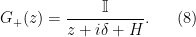
Definition 2 Let be an hermitian matrix. Then we define the retarded green’s function to be

and the advanced green’s function to be

Green’s function are useful for a variety of reasons, usually because they are easier to study than the eigenvalues and eigenfunctions directly. We have the following

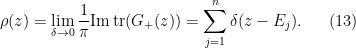
Lemma 3 Let be an hermitian matrix. Then the eigenvalue density function , where are the eigenvalues of and is the Dirac delta function, is given by

(The eigenvalue density function has a delta-function spike at the location of each one of the eigenvalues of .)

Proof: Let’s write out he green’s functions in the eigenbasis of and take the trace: we get

so that

and thus

Taking the limit and using the fact that gives us

We’re now going to use proposition 1 to work out the averaged eigenvalue density function. Before we do we have the following corollary of proposition 1.

Corollary 4 Let be the system (2). Then

where

 

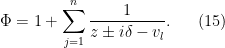
Now we can present the first main result

Proposition 5 Let be the system (2). Then the averaged eigenvalue density (i.e. the eigenvalue density function averaged over the disorder) is given by

where

 

Proof: First note that

We write

To work out the averaged eigenvalue density we take the expectation over the s:

Using the fact that gives us the result, upon writing .

That’s it for today: I spent most of the day making stupid mistakes (eg. working out exact expressions for which couldn’t possibly have ever worked.)

In future posts we’ll take a look at the small- asymptotics of — we know exactly what looks like at , i.e. , because we know the eigenvalues of when . I’m not sure what the best method is to get at the asymptotics at the moment: possibly fixing to be small and doing some contour integrals…?