A quantum generalisation of Talagrand’s inequality

Talagrand’s inequality places nontrivial bounds on the growth of the set of strings which are hamming distance ${k}$ away from some subset of strings. In these notes we formulate a quantum generalisation of Talagrand’s inequality which places bounds on the growth of the dimension of the subspace ${A}$ formed by taking the join of all subspaces which are different from ${A}$ in at most ${k}$ places.

The results in this post are joint work with Andreas Winter.

1. Introduction

High- (and infinite-) dimensional spaces often have counterintuitive properties. One property of certain high-dimensional geometric spaces, which has received a great deal of attention over the years, is the concentration of measure phenomenon (see the books of Milman and Schechtman and Ledoux and Talagrand).

To explain concentration of measure I’ll use the classical example of the ${(n-1)}$ -dimensional sphere ${S^{n-1} = \{(x_1, x_2, \ldots, x_n) \in \mathbb{R}^n\,|\, \|\mathbf{x}\|^2 =1\}}$ . There is a natural metric ${d(\mathbf{x}_0, \mathbf{x}_1)}$ on ${S^{n-1}}$ given by the geodesic distance which measures the length of the shortest arc connecting ${\mathbf{x}_0}$ and ${\mathbf{x}_1}$ (which is always part of a great circle). Let ${\mu}$ be the uniform (haar) measure on ${S^{n-1}}$ . Suppose that ${A}$ is a measurable subset of ${S^{n-1}}$ with measure ${\mu(A) = 1/2}$ and denote by ${A_{\epsilon} = \{\mathbf{x}\,|\, d(\mathbf{x}, A) \le \epsilon\}}$ (i.e., the “fattening” of ${A}$ ). Now the isoperimetric inequality (see appendix I of Milman and Schechtman) says that

Theorem 1 For each ${0 < a < 1}$ and ${\epsilon > 0}$ , ${\mbox{min}\{\mu(A_{\epsilon})\,|\, A\subseteq S^{n-1}, \mu(A) = a\}}$ exists and is attained on ${A_0}$ — a cap with the correct measure (i.e., ${A_0 = B(\mathbf{x}_0, r)}$ for any ${\mathbf{x}_0 \in S^{n-1}}$ and ${r}$ such that ${\mu(B(r))}$ , where ${B(r) = B(\mathbf{x}_0,r) = \{\mathbf{x}\,|\, d(\mathbf{x}, \mathbf{x}_0) \le r\}}$ ).

When ${a=1/2}$ — in which case ${A_0}$ is the half sphere — we get the following

Corollary 2 If ${A\subset S^{n+1}}$ with ${\mu(A) \ge 1/2}$ then ${\mu(A_\epsilon) \ge 1-\sqrt{\frac{\pi}{8}}e^{-\epsilon^2n/2}}$ .

Now, before I show you the proof — which is elementary(!), let’s work out what this is saying: for really high-dimensional spheres, if you start with a half sphere and add in all the points a distance ${O(1/\sqrt{n})}$ then you end up with a subset that basically has the same volume as ${S^{n-1}}$ . That is, adding all the points a vanishingly small (in ${n}$ ) distance away from the equator captures all the volume. Thus we say that all the measure on ${S^{n-1}}$ is concentrated near the equator and that the poles don’t contribute very much at all. Weird. (Compare with the 3d picture below, where, obviously, lots of volume lives near the poles.)

Proof: Obviously, by theorem 1, we only need to evaluate ${\mu(B(\pi/2+\epsilon))}$ . Now the volume of ${S_\theta}$ , the set of points on ${S^{n+1}}$ which are a distance ${\theta}$ from ${B(1/2)}$ (an ${n}$ -dimensional sphere of radius ${\cos(\theta)}$ ) is proportional to ${\cos^{n}(\theta)}$ . As Milman and Schechtman say, you should draw a picture. Thus we learn that

$\displaystyle h(\epsilon, n) = \mu(B(\pi/2+\epsilon)) = \frac{\int_{-\pi/2}^{\epsilon} \cos^n(\theta)d\theta}{\int_{-\pi/2}^{\pi/2} \cos^n(\theta)d\theta}.$

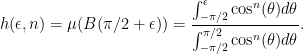
Notice that the important quantity is ${I_n = \int_0^{\pi/2} \cos^n(\theta)d\theta}$ . Now it’s relatively easy to get the desired answer: we need to use the inequality ${\cos(t) \le e^{-t^2/2}}$ and a change of variables ${\theta = \tau/\sqrt{n}}$ :

$\displaystyle 1-h(\epsilon, n) = \frac{1}{2I_n}\int_{\epsilon}^{\pi/2}d\theta \le \frac{\sqrt{\pi/2}e^{-\epsilon^2 n/2}}{2\sqrt{n}I_n} \cos^n(\theta).$

(I’ve skipped some elementary calculations here.) Note that ${\sqrt{n}I_n \ge 1}$ and so

$\displaystyle 1-h(\epsilon,n) \le \sqrt{\frac{\pi}{8}}e^{-\epsilon^2n/2}.$

◻

The concentration of measure phenomenon plays a major role in several fields, including, the asymptotic theory of finite-dimensional Banach spaces, Riemannian geometry, and quantum information theory. It is near ubiquitous in spaces with some kind of product structure: it holds for the ${(n-1)}$ -cube (which is homeorphic to ${S^{n-1}}$ ). Additionally, and this is the result we aim to generalise, it holds for the discrete ${(n-1)}$ -cube of all strings of ${n-1}$ zeros and ones with the hamming distance as the metric. This is the setting of Talagrand’s inequality which is proved in great generality and puissance in Talagrand’s big paper (see Alon and Spencer for a simple exposition of the basic inequality).

In these notes we generalise Talagrand’s inequality to the quantum setting where the role of a subset ${A}$ is played by a subspace and the role of the (product) measure ${\mu}$ is played by a product quantum state (density operator) ${\rho = \sigma\otimes \sigma \otimes \cdots \sigma}$ .

2. The quantum hamming ball

We define ${[n]}$ to be the set ${\{1, 2, \ldots, n\}}$ .

Let ${\mathcal{H}}$ be a hilbert space. If ${Y}$ is a subspace of ${\mathcal{H}}$ then we write ${P(Y)}$ for the corresponding projection onto ${Y}$ ; where obvious, we’ll frequently use ${Y}$ to refer to both the subspace ${Y}$ and the projection ${P(Y)}$ .

Given any family ${\{Y_\alpha\}}$ of subspaces of ${\mathcal{H}}$ , there is a greatest subspace ${\bigwedge_\alpha Y_\alpha}$ that is contained in each ${Y_\alpha}$ and a smallest closed subspace, the join, ${\bigvee_\alpha Y_\alpha}$ that contains each ${Y_\alpha}$ . Specifically, ${\bigwedge_\alpha Y_\alpha}$ is ${\bigcap_{\alpha}Y_\alpha}$ while ${\bigvee_\alpha Y_\alpha}$ is the subspace ${[\bigcup_{\alpha}Y_\alpha]}$ generated by ${\bigcup_{\alpha}Y_\alpha}$ . For each family of projections ${\{P_\alpha\}}$ we write ${\bigwedge_\alpha P_\alpha}$ and ${\bigvee_\alpha P_\alpha}$ for the projections onto the corresponding subspaces ${\bigwedge_\alpha P_\alpha(\mathcal{H})}$ and ${\bigvee_\alpha P_\alpha(\mathcal{H})}$ , respectively. Finally, if ${A}$ is a positive semidefinite (hence, hermitian) operator we define the range of ${A}$ to be the subspace

$\displaystyle \mbox{range}\left(A\right) = \lim_{m\rightarrow\infty} A^{\frac1m}. \ \ \ \ \ (1)$

Throughout these notes our hilbert space ${\mathcal{H}}$ will be that of ${n}$ qudits: ${\mathcal{H} \cong (\mathbb{C}^d)^{\otimes n}}$ , although, we’ll mostly assume ${d}$ is 2 whenever the generalisation to higher ${d}$ is obvious.

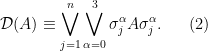
To begin we need to define what is meant by the quantum hamming ball. We are going to define the quantum hamming ball in a fashion similar to the classical definition based on displacement operators. Thus, for any projection ${A}$ , we define the displacement operator:

$\displaystyle \mathcal{D}(A) \equiv \bigvee_{j=1}^n\bigvee_{\alpha = 0}^3 \sigma_j^\alpha A \sigma_j^{\alpha}. \ \ \ \ \ (2)$

We also define the ${k}$ th displacement operator via

$\displaystyle \mathcal{D}^{(j)}(A) \equiv \bigvee_{j_1 < j_2 < \ldots < j_k}\bigvee_{\alpha_1, \alpha_2, \ldots, \alpha_k = 0}^3 (\sigma_{j_1}^{\alpha_1}\otimes \sigma_{j_2}^{\alpha_2} \otimes \cdots \otimes\sigma_{j_k}^{\alpha_k}) A (\sigma_{j_1}^{\alpha_1}\otimes \sigma_{j_2}^{\alpha_2} \otimes \cdots \otimes\sigma_{j_k}^{\alpha_k}). \ \ \ \ \ (3)$

Note that ${\mathcal{D}^{(j)}(A)}$ is not a linear operator.

It is relatively easy to establish the following lemma

Lemma 3 Let ${A}$ be a subspace. Then

$\displaystyle \mathcal{D}^{(j)}(A) = {\mathcal{D}\circ\mathcal{D}\circ \cdots \circ \mathcal{D}}(A). \ \ \ \ \ (4)$

Proof: The result follows upon noting that the hilbert space join operation, also known as the subspace sum operation, is associative: ${A\vee (B\vee C) = (A\vee B)\vee C}$ . ◻

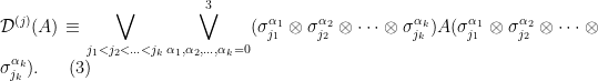
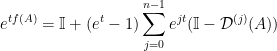
Remark 4 Note that the space of all subspaces of ${\mathcal{H}}$ does not form a lattice under the subspace join and intersection operations.

Using the displacement operator we are able to make sense of the subspace ${A_t}$ , the “fattening” of ${A}$ , which includes all quantum states which are exactly a distance ${t}$ away from ${A}$ :

$\displaystyle A_t \equiv \mathcal{D}^{(t)}(A) \wedge (\mathbb{I}-\mathcal{D}^{(t-1)}(A)), \quad t\ge 1,$

which is equivalent to

$\displaystyle A_t = \mathcal{D}^{(t)}(A) - \mathcal{D}^{(t-1)}(A), \quad t\ge 1.$

where the second inequality follows because the two projections commute: ${[\mathcal{D}^{(t)}(A), \mathcal{D}^{(t-1)}(A)] = 0}$ . We also define ${A_0 \equiv A}$ .

Example 1 Let ${|\psi\rangle = |000\rangle}$ , then

$\displaystyle \mathcal{D}(|\psi\rangle\langle \psi|) = \mbox{span}\{|000\rangle, |100\rangle, |010\rangle, |001\rangle\}. \ \ \ \ \ (5)$

We now come to the quantum hamming distance. To make sense of how far a quantum state ${|\phi\rangle}$ is from a subspace ${A}$ we construct the following positive semidefinite operator

$\displaystyle f(A) = \sum_{j=0}^n jA_j. \ \ \ \ \ (6)$

Given an arbitrary quantum state ${|\phi\rangle}$ we define the quantum hamming distance of ${|\phi\rangle}$ to ${A}$ to be

$\displaystyle f(A, |\phi\rangle) = \langle \phi|f(A)|\phi\rangle. \ \ \ \ \ (7)$

We’ll have occasion to use the following

Lemma 5 (Operator Markov inequality) Let ${A = \sum_{j=1}^d a_j|j\rangle\langle j|}$ be a positive semidefinite operator and ${\rho}$ any density operator. Define

$\displaystyle P_\lambda \equiv \sum_{j=1}^d \chi(a_j-\lambda) |j\rangle\langle j| \ \ \ \ \ (8)$

where ${\chi(x)=\begin{cases}0,&\quad x\le0\\1,&\quad x>0\end{cases}}$ . Then

$\displaystyle \mbox{tr}(\rho P_\lambda) \le \frac{1}{\lambda}\mbox{tr}(\rho A). \ \ \ \ \ (9)$

Proof: Notice that

$\displaystyle \lambda P_\lambda \le A, \ \ \ \ \ (10)$

and taking the trace of both sides against ${\rho}$ gives us

$\displaystyle \mbox{tr}(\rho P_\lambda) \le\frac{1}{\lambda}\mbox{tr}(\rho A). \ \ \ \ \ (11)$

◻

Before we move on to the next section we’ll prove a simple but useful lemma concerning the ranges of sums of positive semidefinite operators.

Lemma 6 Let ${M = A+B}$ , where ${A}$ and ${B}$ are two bounded positive semidefinite operators. Then

$\displaystyle R_M = R_A\vee R_B, \ \ \ \ \ (12)$

where ${R_M =\mbox{range}(M)}$ , ${R_A = \mbox{range}(A)}$ , and ${R_B =\mbox{range}(B)}$ .

Proof: To prove this result we study the complement ${\overline{R_M}}$ of ${R_M}$ . A vector ${|\phi\rangle}$ is in ${\overline{R_M}}$ if and only if ${M|\phi\rangle = 0}$ . That is, if and only if ${\langle \phi|M|\phi\rangle = 0}$ . (Why? Consider that ${\langle \phi|M|\phi\rangle = 0 = \|\sqrt{M}|\phi\rangle\|^2}$ implies that ${\sqrt{M}|\phi\rangle = 0}$ . Applying ${\sqrt{M}}$ to both sides gives the result.) Now suppose that ${|\phi\rangle}$ is in ${\overline{R_M}}$ . This means that ${\langle \phi|M|\phi\rangle = 0 = \langle \phi|A|\phi\rangle+ \langle \phi|B|\phi\rangle}$ , i.e., ${A|\phi\rangle = 0 = B|\phi\rangle}$ . This occurs if and only if ${|\phi\rangle}$ is in both of ${\overline{R_A}}$ and ${\overline{R_B}}$ , i.e., ${(\overline{R_A}\wedge \overline{R_B})|\phi\rangle = |\phi\rangle}$ . But this means that ${\overline{R_M} = \overline{R_A}\wedge \overline{R_B}}$ or, after taking complements, that ${R_M = R_A \vee R_B}$ . ◻

3. The quantum Talagrand inequality

In these notes we aim to prove the following

Proposition 7 Let ${A}$ be a projection and let ${\sigma}$ be a single-qubit density operator. Then

$\displaystyle \mbox{tr}(\sigma^{\otimes n} e^{tf(A)}) \le \frac{a(t)^n}{\mbox{tr}(\sigma^{\otimes n} A)}$

$\displaystyle \le \frac{1}{\mbox{tr}(\sigma^{\otimes n} A)}e^{\frac{nt^2}{4}},$

where

$\displaystyle a(t) = \frac12 + \frac{\cosh(t)}{2}. \ \ \ \ \ (13)$

The proof of this proposition relies on the following seven lemmas.

Lemma 8 Let ${A}$ be a projection. Then

$\displaystyle e^{tf(A)} = \mathbb{I} + (e^t-1)\sum_{j=0}^{n-1} e^{jt}(\mathbb{I} - \mathcal{D}^{(j)}(A)). \ \ \ \ \ (14)$

Proof:

$\displaystyle e^{tf(A)} = \sum_{j=0}^{n} e^{jt} A_j$

$\displaystyle = \sum_{j=0}^{n} e^{jt} (\mathcal{D}^{(j)}(A) - \mathcal{D}^{(j-1)}(A))$

$\displaystyle = e^{nt}\mathbb{I} + \sum_{j=0}^{n-1} e^{jt} \mathcal{D}^{(j)}(A) - \sum_{j=1}^{n} e^{jt} \mathcal{D}^{(j-1)}(A)$

$\displaystyle = e^{nt}\mathbb{I} + (1-e^t)\sum_{j=0}^{n-1} e^{jt} \mathcal{D}^{(j)}(A)$

$\displaystyle = \mathbb{I} + (1-e^t)\sum_{j=0}^{n-1} e^{jt}(\mathcal{D}^{(j)}(A)-\mathbb{I})$

$\displaystyle = \mathbb{I} + (e^t-1)\sum_{j=0}^{n-1} e^{jt}(\mathbb{I}-\mathcal{D}^{(j)}(A)),$

where we’ve used ${\mathcal{D}^{n}(A) = \mathbb{I}}$ in the third line and the fact that ${(1-e^{t})\sum_{j=0}^{n-1} e^{jt} = (1-e^{nt})}$ in the fifth line. ◻

Definition 9 Let ${A}$ be a projection and let ${|\omega\rangle}$ be a single-qubit state. We define ${A(\omega)}$ to be a projection on ${(\mathbb{C}^2)^{\otimes n-1}}$ which has the largest dimension so that

$\displaystyle A(\omega)\otimes |\omega\rangle\langle \omega| \le A, \ \ \ \ \ (15)$

where the inequality refers to the positive semidefinite ordering. We also define the projection ${B}$ on ${(\mathbb{C}^2)^{\otimes n-1}}$ to be the range of the partial trace over the ${n}$ th qubit of ${A}$ :

$\displaystyle B = \mbox{range}\left(\frac12\mbox{tr}_{n}(A)\right). \ \ \ \ \ (16)$

Lemma 10 Let ${A}$ be a projection and let ${|\omega\rangle}$ be a single-qubit state. We have that

$\displaystyle \mathcal{D}^{(j)}(A(\omega)) \le \mathbb{I}\otimes\langle \omega|(\mathcal{D}^{(j)}(A))\mathbb{I}\otimes|\omega\rangle. \ \ \ \ \ (17)$

Proof: We begin by observing that

$\displaystyle \mathcal{D}^{(j)}(A(\omega))\otimes |\omega\rangle\langle\omega| \le \mathcal{D}^{(j)}(A(\omega)\otimes |\omega\rangle\langle\omega|)$

$\displaystyle \le \mathcal{D}^{(j)}(A).$

From this operator inequality we obtain

$\displaystyle \mathbb{I}\otimes \langle \omega|(\mathcal{D}^{(j)}(A(\omega))\otimes |\omega\rangle\langle\omega|)\mathbb{I}\otimes |\omega\rangle \le \mathbb{I}\otimes\langle \omega|(\mathcal{D}^{(j)}(A))\mathbb{I}\otimes|\omega\rangle, \ \ \ \ \ (18)$

which is the desired result. ◻

Lemma 11 Let ${A}$ be a projection and let ${|\omega\rangle}$ be a single-qubit state. We have that

$\displaystyle \mathbb{I}\otimes\langle \omega|\left(e^{tf(A)}\right)\mathbb{I}\otimes|\omega\rangle \le e^{tf(A(\omega))}, \ \ \ \ \ (19)$

Proof: Consider

$\displaystyle \mathbb{I}\otimes\langle \omega|\left(e^{tf(A)}\right)\mathbb{I}\otimes|\omega\rangle = \mathbb{I} + (e^t-1)\sum_{j=0}^{n-1} e^{jt}(\mathbb{I}-\mathbb{I}\otimes\langle \omega|(\mathcal{D}^{(j)}(A))\mathbb{I}\otimes|\omega\rangle)$

$\displaystyle \le \mathbb{I} + (e^t-1)\sum_{j=0}^{n-1} e^{jt}(\mathbb{I}-\mathcal{D}^{(j)}(A(\omega)))$

$\displaystyle = e^{tf(A(\omega))}.$

◻

In the next lemma we prove a crucial structure result concerning joins of locally displaced subspaces.

Lemma 12 Let ${A}$ be a projection, and ${B}$ be as in Definition 9. Then

$\displaystyle \bigvee_{\alpha=0}^3 \sigma_n^\alpha A \sigma_n^\alpha = B\otimes \mathbb{I}. \ \ \ \ \ (20)$

Proof: First, thanks to Lemma 6, we have that if

$\displaystyle A = \sum_{j=1}^m |\phi_j\rangle\langle\phi_j| \ \ \ \ \ (21)$

then

$\displaystyle B = \bigvee_{j=1}^m S_j, \ \ \ \ \ (22)$

where ${S_j = \mbox{range}(\frac{1}{2}\mbox{tr}_n(\phi_j))}$ . Thus we learn that ${B\otimes \mathbb{I}}$ is generated by linear combinations of vectors of the form ${|u\rangle_{[n-1]}|\omega\rangle_n}$ , where ${|\omega\rangle_n}$ is an arbitrary single-qubit state and ${|u\rangle_{[n-1]}}$ is an eigenvector of ${\frac12\mbox{tr}_n(\phi_j)}$ for some ${j\in [m]}$ .

Now, we’re going to show that ${\bigvee_{\alpha=0}^3 \sigma_n^\alpha A \sigma_n^\alpha \ge B\otimes \mathbb{I}}$ . Suppose that ${|u\rangle_{[n-1]}|\omega\rangle_n}$ is a vector in ${B\otimes \mathbb{I}}$ . It turns out that ${|u\rangle_{[n-1]}|\omega\rangle_n}$ lies in ${\bigvee_{\alpha=0}^3 \sigma_n^\alpha A \sigma_n^\alpha}$ : suppose that ${|u\rangle}$ arises as an eigenvector (corresponding to a nonzero eigenvalue) of ${\frac12\mbox{tr}_n(\phi)}$ for ${|\phi\rangle}$ in ${A}$ . Then

$\displaystyle |\psi\rangle = \sum_{\alpha=0}^3 c_\alpha \sigma_n^\alpha |\phi\rangle \ \ \ \ \ (23)$

lies in the subspace ${\bigvee_{\alpha=0}^3 \sigma_n^\alpha A \sigma_n^\alpha}$ for all ${c_\alpha}$ . Now write the Schmidt decomposition of ${|\phi\rangle}$ as

$\displaystyle |\phi\rangle = \sqrt{q}|u\rangle_{[n-1]}|v\rangle_n + |\phi_\perp\rangle. \ \ \ \ \ (24)$

To show the desired inclusion we apply the projector ${P_v = \mathbb{I}_{[n-1]}\otimes|v\rangle_n\langle v|}$ and then the rotation ${U_\omega = \mathbb{I}_{[n-1]}\otimes|\omega\rangle_n\langle v|}$ to ${|\phi\rangle}$ :

$\displaystyle |u\rangle|\omega\rangle = U_\omega P_v |\phi\rangle. \ \ \ \ \ (25)$

Because ${\sigma_n^\alpha}$ is a complete orthonormal basis we have that ${U_\omega P_v = \sum_{\alpha=0}^3 c_\alpha \mathbb{I}_{[n-1]}\otimes \sigma_n^\alpha}$ for some ${c_\alpha}$ so that

$\displaystyle |u\rangle|\omega\rangle = \sum_{\alpha=0}^3 c_\alpha \sigma_n^\alpha|\phi\rangle, \ \ \ \ \ (26)$

so that ${|u\rangle|\omega\rangle}$ lies in ${\bigvee_{\alpha=0}^3 \sigma_n^\alpha A \sigma_n^\alpha}$ for all ${|\omega\rangle}$ , and hence the subspace ${|u\rangle\langle u|\otimes \mathbb{I}}$ lies in ${\bigvee_{\alpha=0}^3 \sigma_n^\alpha A \sigma_n^\alpha}$ . Since ${B\otimes \mathbb{I}}$ is generated by all vectors of this form, we have the desired inclusion.

The reverse inclusion is easy: applying ${B\otimes \mathbb{I}}$ to a any vector ${|\psi\rangle}$ in ${\bigvee_{\alpha=0}^3 \sigma_n^\alpha A \sigma_n^\alpha}$ and using the fact that ${|\psi\rangle = \sum_{j=1}^k c_j \sigma_n^{\alpha_j} |\phi_j\rangle}$ , where ${|\phi_j\rangle}$ lie in ${A}$ , and that ${B\otimes \mathbb{I} \ge A}$ gives us the desired result. ◻

Lemma 13 Let ${A}$ be a projection, and ${B}$ be defined as in Definition 9. Then

$\displaystyle \mathcal{D}^{(j)}(A) \ge \mathcal{D}^{(j-1)}(B)\otimes \mathbb{I}, \quad j\ge 1. \ \ \ \ \ (27)$

Proof: We prove this lemma by induction. We start with the base case

$\displaystyle \mathcal{D}^{(1)}(A) \ge B\otimes \mathbb{I}, \ \ \ \ \ (28)$

which may be shown as follows. Firstly, note that

$\displaystyle \mathcal{D}^{(1)}(A) \ge \bigvee_{\alpha=0}^3 \sigma_n^\alpha A \sigma_n^\alpha. \ \ \ \ \ (29)$

Notice that this is in the form covered by the previous lemma, so that we have

$\displaystyle \mathcal{D}^{(1)}(A) \ge B\otimes \mathbb{I} \ \ \ \ \ (30)$

as required. We can now complete the proof by demonstrating the inductive step:

$\displaystyle \mathcal{D}^{(j)}(A) = \mathcal{D}^{(1)}(\mathcal{D}^{(j-1)}(A))$

$\displaystyle \ge \mathcal{D}^{(1)}(\mathcal{D}^{(j-2)}(B)\otimes \mathbb{I})$

$\displaystyle = \mathcal{D}^{(j-1)}(B)\otimes \mathbb{I}.$

◻

Lemma 14 Let ${A}$ be a projection. Then

$\displaystyle e^{tf(A)} \le e^t(e^{tf(B)}\otimes\mathbb{I}). \ \ \ \ \ (31)$

Proof: We use Lemma 8 and Lemma 13:

$\displaystyle e^{tf(A)} = \mathbb{I} + (e^t-1)\sum_{j=0}^{n-1} e^{jt}(\mathbb{I} - \mathcal{D}^{(j)}(A))$

$\displaystyle \le \mathbb{I} + (e^t-1)\mathbb{I} + (e^t-1)\sum_{j=1}^{n-1} e^{jt}(\mathbb{I} - \mathcal{D}^{(j-1)}(B)\otimes \mathbb{I})$

$\displaystyle = e^t\mathbb{I} + (e^t-1)\sum_{j=0}^{n-2} e^{(j+1)t}(\mathbb{I} - \mathcal{D}^{(j)}(B)\otimes \mathbb{I})$

$\displaystyle = e^t\left(\mathbb{I} + (e^t-1)\sum_{j=0}^{n-2} e^{jt}(\mathbb{I} - \mathcal{D}^{(j)}(B))\right)\otimes \mathbb{I}$

$\displaystyle = e^t(e^{tf(B)}\otimes\mathbb{I}).$

◻

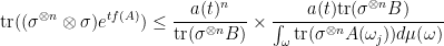
Lemma 15 Let ${A}$ be a projection and let ${\sigma = \sum_{j=1}^d p_j|\omega_j\rangle\langle \omega_j|}$ be a single-qubit state. We have that

$\displaystyle \mbox{tr}_n((\mathbb{I}_{[n-1]}\otimes \sigma) e^{tf(A)})\le \sum_{j=1}^d p_j e^{tf(A(\omega_j))}, \ \ \ \ \ (32)$

and

$\displaystyle \mbox{tr}((\mathbb{I}_{[n-1]}\otimes \sigma) e^{tf(A)})\le e^{(t+1)f(B)}. \ \ \ \ \ (33)$

Proof: The proof follows straightforwardly from Lemma 19 and Lemma 14 ◻

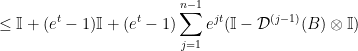
We need one final lemma before proving the proposition; this lemma appears in Talagrand’s big paper:

Lemma 16 Consider a measurable function ${g}$ on a measure space ${\Omega}$ . Assume ${0\le g \le 1}$ . Then we have

$\displaystyle \int_\Omega \min\left(e^t, \frac{1}{g(\omega)}\right)d\mu(\omega)\int_\Omega g(\omega)d\mu(\omega) \le a(t). \ \ \ \ \ (34)$

Proof: [Proof of Proposition 7] We proceed by induction on ${n}$ (the base case follows from the preceeding lemma). Suppose the result has been proved for ${n}$ . We prove it for ${n+1}$ as follows. Let ${\sigma = \sum_{j=1}^d p_j|\omega_j\rangle\langle \omega_j|}$ . By Lemma 15 we have that

$\displaystyle \mbox{tr}((\sigma^{\otimes n}\otimes \sigma) e^{tf(A)}) \le \sum_{j=1}^d p_j\mbox{tr}(\sigma^{\otimes n}e^{tf(A(\omega_j))}) \le \sum_{j=1}^d p_j\frac{a(t)^n}{\mbox{tr}(\sigma^{\otimes n}A(\omega_j))} \ \ \ \ \ (35)$

and

$\displaystyle \mbox{tr}((\sigma^{\otimes n}\otimes \sigma) e^{tf(A)}) \le e^t\frac{a(t)^n}{\mbox{tr}(\sigma^{\otimes n} B)}. \ \ \ \ \ (36)$

Thus

$\displaystyle \mbox{tr}((\sigma^{\otimes n}\otimes \sigma) e^{tf(A)}) \le \frac{a(t)^n}{\mbox{tr}(\sigma^{\otimes n} B)}\int_\Omega \min\left\{e^t, \frac{1}{g(\omega)} \right\} d\mu(\omega), \ \ \ \ \ (37)$

where we’ve defined (implicitly) the discrete measure space ${\Omega = (\{\omega_j\}_{j=1}^d, \mu)}$ , with ${\mu(\omega_j) = p_j}$ and the measurable function

$\displaystyle g(\omega_j) = \frac{\mbox{tr}(\sigma^{\otimes n}A(\omega_j))}{\mbox{tr}(\sigma^{\otimes n} B)}. \ \ \ \ \ (38)$

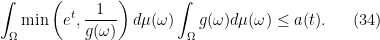
Applying Lemma 16 gives

$\displaystyle \mbox{tr}((\sigma^{\otimes n}\otimes \sigma) e^{tf(A)}) \le \frac{a(t)^n}{\mbox{tr}(\sigma^{\otimes n} B)} \times \frac{a(t) \mbox{tr}(\sigma^{\otimes n} B)}{\int_\omega\mbox{tr}(\sigma^{\otimes n}A(\omega_j))d\mu(\omega)}$

$\displaystyle = \frac{a(t)^{n+1}}{\mbox{tr}(\sigma^{\otimes (n+1)}A)}.$

To complete the proof we now show that ${a(t) \le e^{\frac{t^2}{4}}}$ . We begin by taking the logarithm of ${a(t)}$ :

$\displaystyle c(t) = \log\left(\frac{1}{2}+\frac{\cosh(t)}{2}\right). \ \ \ \ \ (39)$

Next we differentiate ${c(t)}$ to give

$\displaystyle \frac{dc(t)}{dt} = \frac{1}{2}\left(\frac{1}{2}+\frac{\cosh(t)}{2}\right)^{-1}\sinh(t)$

$\displaystyle = \frac{\sinh(t)}{1+\cosh(t)}$

$\displaystyle \le \frac{t}{2}.$

Now integrate this differential inequality with the initial condition ${c(0) = 0}$ to obtain

$\displaystyle c(t) \le \frac{t^2}{4}, \ \ \ \ \ (40)$

and hence ${a(t) \le e^{\frac{t^2}{4}}}$ . ◻

Corollary 17 Let ${A}$ be a subspace. Then

$\displaystyle 1- \frac{e^{-\frac{k^2}{n}}}{\mbox{tr}(\sigma^{\otimes n} A)} \le \mbox{tr}(\sigma^{\otimes n} \mathcal{D}^{(k-1)}(A)). \ \ \ \ \ (41)$

Proof: We use the operator Markov inequality Lemma 5, as applied to the positive semidefinite operator ${e^{tf(A)}}$ :

$\displaystyle e^{tk} (\mathbb{I}-\mathcal{D}^{(k-1)}(A)) \le e^{tf(A)}. \ \ \ \ \ (42)$

Taking the trace of both sides with respect to ${\sigma^{\otimes n}}$ gives

$\displaystyle \mbox{tr}(\sigma^{\otimes n}(\mathbb{I}-\mathcal{D}^{(k-1)}(A))) \le e^{-tk}\mbox{tr}(\sigma^{\otimes n}e^{tf(A)}). \ \ \ \ \ (43)$

Applying the quantum Talagrand inequality gives

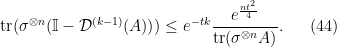
$\displaystyle \mbox{tr}(\sigma^{\otimes n}(\mathbb{I}-\mathcal{D}^{(k-1)}(A))) \le e^{-tk} \frac{e^{\frac{nt^2}{4}}}{\mbox{tr}(\sigma^{\otimes n} A)}. \ \ \ \ \ (44)$

Choosing ${t=2k/n}$ yields

$\displaystyle \mbox{tr}(\sigma^{\otimes n}(\mathbb{I}-\mathcal{D}^{(k-1)}(A))) \le \frac{e^{-\frac{k^2}{n}}}{\mbox{tr}(\sigma^{\otimes n} A)} \ \ \ \ \ (45)$

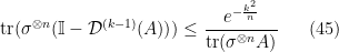
which, upon rearranging, gives the desired result. ◻

Discussion

The main result of this post is proposition 7, but the inequality that actually best mimics Talagrand’s inequality is corollary 17. Now, what people call Talagrand’s inequality isn’t actually either result! “Talagrand’s inequality” refers to a much more general result which applies not only to the hamming distance but to much more general distance measures. At the moment it is unclear (to me, at least) how to generalise the proof here to the case where the “quantum hamming distance” (7) is replaced with something more general…

This entry was posted on Friday, February 13th, 2009 at 11:41 am and is filed under concentration of measure. You can follow any responses to this entry through the RSS 2.0 feed. You can leave a response, or trackback from your own site.

2 Responses to A quantum generalisation of Talagrand’s inequality

Tasos Zouzias says:

February 27, 2010 at 12:52 am

Looks very interesting. Do you have any draft on this result other than this post?

Thanks,
Tasos

Reply
- tobiasosborne says:
  
  April 5, 2010 at 1:51 pm
  
  Dear Tasos Zouzias,
  
  Many thanks for your interest!
  
  Unfortunately the post this is the only draft available of this result at the current time. I’ll let you know if/when I come to write it up for publication.
  
  Best wishes!
  
  Sincerely,
  Tobias
  
  Reply

Tobias J. Osborne's research notes