The variational principle in quantum mechanics, lecture 5

1. Lecture 5: Mean-field theory and the Gross-Pitaevskii equation

In the previous lecture we saw two applications of the variational principle to the class of product states and fermionic gaussian states, respectively. In both cases we obtained an effective equation for the ground-state properties involving only a single effective particle (a single spin in the first case and a single majorana fermion in the second case).

In this lecture we continue our study of mean-field theory in the bosonic setting, in particular to the description of Bose-Einstein condensates. Here we find a similar result: we’ll obtain a nonlinear effective equation for the condensate in terms of a single effective particle degree of freedom. Before we do this we need to review some of the formalism for the description of quantum fields and coherent states.

The pdf version of the notes can be found here.

2. Quantum fields

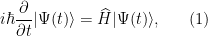
Recall that in lecture 3 we showed that the second-quantised many particle Schrödinger equation for the abstract state vector ${|\Psi(t)\rangle}$ admitted the form

$\displaystyle i\hbar \frac{\partial}{\partial t}|\Psi(t)\rangle = \widehat{H}|\Psi(t)\rangle, \ \ \ \ \ (1)$

where the operator ${\widehat{H}}$ is given by

$\displaystyle \widehat{H} = \sum_{j,k} c_j^\dag \langle j|T|k\rangle c_k + \frac12 \sum_{j,k,l,m} c_j^\dag c_k^\dag \langle jk|V|lm\rangle c_l c_m. \ \ \ \ \ (2)$

where ${c_k}$ and ${c_k^\dag}$ are the annihilation and creation operators, respectively, for a complete set of single-particle wave functions ${\psi_k(x)}$ . (We consider the bosonic and fermionic cases in parallel, so that ${c_k}$ and ${c_k^\dag}$ either satisfy the CCR or CAR, respectively.)

It is convenient to introduce the following field operators

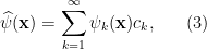
$\displaystyle \widehat{\psi}(\mathbf{x}) = \sum_{k=1}^\infty \psi_k(\mathbf{x}) c_k, \ \ \ \ \ (3)$

and

$\displaystyle \widehat{\psi}^\dag(\mathbf{x}) = \sum_{k=1}^\infty \overline{\psi}_k(\mathbf{x}) c_k^\dag. \ \ \ \ \ (4)$

These operators satisfy the simple (anti)commutation relations, following from the completeness relation:

$\displaystyle [\widehat{\psi}(\mathbf{x}), \widehat{\psi}^\dag(\mathbf{y})]_{\pm} = \sum_{k} \psi_k(\mathbf{x})\overline{\psi}_k(\mathbf{y}) = \delta(\mathbf{x}-\mathbf{y})$ ,

and

$\displaystyle [\widehat{\psi}(\mathbf{x}), \widehat{\psi}(\mathbf{y})]_{\pm} = [\widehat{\psi}^\dag(\mathbf{x}), \widehat{\psi}^\dag(\mathbf{y})]_{\pm} = 0,$

where the subscript ${\pm}$ on the brackets denotes commutator/anticommutator depending on whether the system is bosonic/fermionic, respectively.

In these terms the hamiltonian operator may be rewritten as

$\displaystyle \widehat{H} = \int d^3\mathbf{x}\, \widehat{\psi}^\dag(\mathbf{x}) T(\mathbf{x}) \widehat{\psi}(\mathbf{x}) + \frac12\int d^3\mathbf{x}d^3\mathbf{y}\, \widehat{\psi}^\dag(\mathbf{x}) \widehat{\psi}^\dag(\mathbf{y}) V(\mathbf{x}, \mathbf{y})\widehat{\psi}(\mathbf{y}) \widehat{\psi}(\mathbf{x}). \ \ \ \ \ (5)$

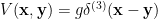
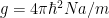
One example that will concern us in the sequel is that of a dilute gas of ${N}$ bosons dominated by low energy two-particle ${s}$ -wave collisions moving in an external potential. In this case we have that ${T(\mathbf{x})}$ is given by ${T(\mathbf{x}) = -\frac{\hbar^2}{2m}\nabla^2+V_{\mbox{ext}}}$ , and ${V(\mathbf{x},\mathbf{y}) = g\delta^{(3)}(\mathbf{x}-\mathbf{y})}$ , where ${g = 4\pi\hbar^2Na/m}$ , so that

$\displaystyle \widehat{H} = \int d^3\mathbf{x}\, \widehat{\psi}^\dag(\mathbf{x}) \left(-\frac{\hbar^2}{2m}\nabla^2+V_{\mbox{ext}}(\mathbf{x})\right) \widehat{\psi}(\mathbf{x}) + \frac{g}2\int d^3\mathbf{x}\, \widehat{\psi}^\dag(\mathbf{x}) \widehat{\psi}^\dag(\mathbf{x}) \widehat{\psi}(\mathbf{x}) \widehat{\psi}(\mathbf{x}). \ \ \ \ \ (6)$

3. Coherent states

We now recall the definition of a coherent state. Suppose that ${a}$ and ${a^\dag}$ are the annihilation and creation operators, respectively, for a single quantum harmonic oscillator satisfying ${[a, a^\dag] = \mathbb{I}}$ , etc. Let ${|0\rangle}$ be the vacuum state which satisfies

$\displaystyle a|0\rangle = 0. \ \ \ \ \ (7)$

Let ${\alpha \in \mathbb{C}}$ and define the displacement operator

$\displaystyle D(a,\alpha) = e^{\alpha a^\dag - \overline{\alpha} a}. \ \ \ \ \ (8)$

This is a unitary operator. One can use the Baker-Campbell-Hausdorff expansion to show that

$\displaystyle D(a,\alpha) = e^{\alpha a^\dag}e^{- \overline{\alpha} a}e^{-\frac12 |\alpha|^2}. \ \ \ \ \ (9)$

A coherent state is then defined to be

$\displaystyle |\alpha\rangle = D(a,\alpha)|0\rangle. \ \ \ \ \ (10)$

These states have the property that

$\displaystyle a|\alpha\rangle = \alpha |\alpha\rangle. \ \ \ \ \ (11)$

The set of coherent states supply an overcomplete basis for hilbert space; we have the completeness relation

$\displaystyle \mathbb{I} = \frac1\pi\int d^2\alpha\, |\alpha\rangle\langle \alpha|. \ \ \ \ \ (12)$

Any coherent state is an example of a gaussian state. However the set of gaussian states is larger than that of coherent states: there exist squeezed states which are also gaussian and which aren’t coherent.

The generalisation to many harmonic oscillators proceeds as follows. Let ${a_j}$ and ${a_j^\dag}$ , ${j = 1, 2, \ldots, N}$ , be the annihilation and creation operators, respectively, for a ${N}$ quantum harmonic oscillators satisfying ${[a_j, a^\dag_k] = \delta_{j,k}\mathbb{I}}$ , ${j,k = 1, 2, \ldots, N}$ . We think of the harmonic oscillators as being arranged in a line.

Let ${\boldsymbol{\alpha} \in \mathbb{C}^n}$ and define

$\displaystyle |\boldsymbol{\alpha}\rangle = D(a,\boldsymbol{\alpha})|0\rangle, \ \ \ \ \ (13)$

where

$\displaystyle D(a,\boldsymbol{\alpha}) = e^{\sum_{j=1}^n\alpha_j a^\dag_j - \overline{\alpha}_j a_j}. \ \ \ \ \ (14)$

The set of states ${\mathcal{V} = \{|\boldsymbol{\alpha}\rangle \,|\, \boldsymbol{\alpha} \in \mathbb{C}^N\}}$ forms a convenient variational class. To see what a variational calculation looks like in this setting we study the following

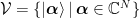
4. Example 1: the Bose-Hubbard model

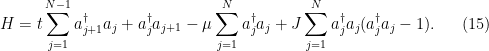
The Bose-Hubbard model is an effective model for bosons hopping in a lattice with repulsive onsite interactions. It can be taken as a model for, e.g., trapped cold atoms moving in the presence of a periodic potential. The hamiltonian is given by

$\displaystyle H = t\sum_{j=1}^{N-1} a_{j+1}^\dag a_j + a_{j}^\dag a_{j+1} -\mu\sum_{j=1}^N a_j^\dag a_j+ J \sum_{j=1}^N a_j^\dag a_j( a_j^\dag a_j - 1). \ \ \ \ \ (15)$

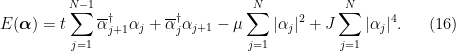
The expectation value ${E(\boldsymbol{\alpha}) = \langle H \rangle}$ of ${H}$ in a coherent state ${|\boldsymbol{\alpha}\rangle}$ is given by

$\displaystyle E(\boldsymbol{\alpha}) = t\sum_{j=1}^{N-1} \overline{\alpha}_{j+1}^\dag \alpha_j + \overline{\alpha}_{j}^\dag \alpha_{j+1} -\mu\sum_{j=1}^N |\alpha_j|^2 + J \sum_{j=1}^N |\alpha_j|^4. \ \ \ \ \ (16)$

Taking the limit ${N\rightarrow\infty}$ and assuming translation invariance gives the following expression for the energy density ${e(\alpha) = E(\boldsymbol{\alpha})/N}$

$\displaystyle e(\alpha) = (2t-\mu)|\alpha|^2 + J |\alpha|^4. \ \ \ \ \ (17)$

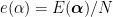
The variation is then over the single complex number ${\alpha = re^{i\phi}}$ :

$\displaystyle \min_{r\ge 0, \phi \in [0,2\pi)} e(re^{i\phi}) = \min_{r\ge 0} (2t-\mu)r^2 + Jr^4. \ \ \ \ \ (18)$

The minimum occurs at ${r=0}$ and

$\displaystyle r = \sqrt{\frac{2(\mu-2t)}{J}}. \ \ \ \ \ (19)$

This solution reflects the fact that if the chemical potential ${\mu}$ is large enough then it is energetically favourable for the system to support a finite density of particles. Unfortunately the translation-invariant version ${\alpha_j = \alpha}$ of our class which we used here is a little too trivial to give good information about the Bose-Hubbard model. The non-translation invariant case is more interesting and gives a better approximation. However, we can no longer find the minimum in compact form.

5. Coherent states for quantum fields

Let ${\widehat{\psi}(\mathbf{x})}$ and ${\widehat{\psi}^\dag(\mathbf{x})}$ be the bosonic field annihilation and creation operators. We define the quantum field displacement operator via

$\displaystyle D(\widehat{\psi}, \phi) \equiv e^{\int d^3\mathbf{x} \, \phi(\mathbf{x})\widehat{\psi}^\dag(\mathbf{x}) - \overline{\phi}(\mathbf{x})\widehat{\psi}(\mathbf{x})}, \ \ \ \ \ (20)$

where ${\phi(\mathbf{x}) \in \mathbb{C}}$ is a complex function. We use the field displacement operator to define a field coherent state ${|\phi\rangle}$ via

$\displaystyle |\phi\rangle = D(\widehat{\psi}, \phi) |\Omega\rangle. \ \ \ \ \ (21)$

Note that a field coherent state obeys

$\displaystyle \widehat{\psi}(\mathbf{x})|\phi\rangle = \phi(\mathbf{x})|\phi\rangle \ \ \ \ \ (22)$

and

$\displaystyle \frac{\partial\widehat{\psi}(\mathbf{x})}{\partial x}|\phi\rangle = \frac{\partial\phi(\mathbf{x})}{\partial x}|\phi\rangle, \ \ \ \ \ (23)$

etc. Exercise: prove this using a Taylor series for the exponential and the commutation relations for the field operators. We now take as our variational class the set

$\displaystyle \mathcal{V} = \{|\phi\rangle \,|\, \phi:\mathbb{R}^3\rightarrow \mathbb{C}\}, \ \ \ \ \ (24)$

where the set of functions ${\phi}$ in the definition of ${\mathcal{V}}$ are taken to be twice-differentiable.

6. Example 2: Bose-Einstein condensates

We apply the variational principle to ${\widehat{H}}$ given in (6) modelling a dilute gas of bosons using the class ${\mathcal{V}}$ ; we obtain the expectation value

$\displaystyle \langle \phi|\widehat{H}|\phi\rangle = \int d^3\mathbf{x}\, \overline{\phi}(\mathbf{x}) \left(-\frac{\hbar^2}{2m}\nabla^2+V_{\mbox{ext}}(\mathbf{x})\right) \phi(\mathbf{x}) + \frac{g}2\int d^3\mathbf{x}\, |\phi(\mathbf{x})|^4. \ \ \ \ \ (25)$

To apply the variational principle we need to extremise ${\langle \phi|\widehat{H}|\phi\rangle}$ by minimising over all ${\phi(\mathbf{x})}$ . This is easy to carry out using variational calculus: the Euler-Lagrange equations give

$\displaystyle 0 = \frac{\delta}{\delta \overline{\phi}(\mathbf{x})}\langle \phi|\widehat{H}|\phi\rangle, \ \ \ \ \ (26)$

which reduce to

$\displaystyle \left(-\frac{\hbar^2}{2m}\nabla^2+V_{\mbox{ext}}(\mathbf{x})\right) \phi(\mathbf{x}) + g |\phi(\mathbf{x})|^2 \phi(\mathbf{x}) = 0. \ \ \ \ \ (27)$

This nonlinear Schrödinger equation is known as the (time-independent) Gross-Pitaevskii equation (GPE). The single-particle solution ${\phi(\mathbf{x})}$ models a Bose-Einstein condensate in an external potential. The nonlinear term models the averaged, or mean-field, interaction with the other particles.

Exercise: make the Thomas-Fermi approximation in the large- ${N}$ limit by neglecting the kinetic energy derivative term in the GPE. What solution do you obtain for ${\phi(\mathbf{x})}$ ? Compare this with the lattice calculation of the previous section.

This entry was posted on Wednesday, May 11th, 2011 at 1:31 pm and is filed under teaching. You can follow any responses to this entry through the RSS 2.0 feed. You can leave a response, or trackback from your own site.

Tobias J. Osborne's research notes