Dynamics of the Anderson model I

In this post I’d like to continue looking at the dynamics of disordered systems. In particular I want to discuss the dynamics of the basic discrete 1D Anderson within the approximation developed in the previous post. As we’ll see, this can be reduced to the solution of a partial integro-differential equation.

1. Dynamics of the discrete Anderson model

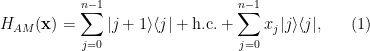
Recall that the hamiltonian for the discrete 1D Anderson model is given by

$\displaystyle H_{AM}(\mathbf{x}) = \sum_{j=0}^{n-1} |j+1\rangle\langle j| + \mbox{h.c.} + \sum_{j=0}^{n-1} x_j |j\rangle\langle j|, \ \ \ \ \ (1)$

where addition is modulo ${n}$ . (We slightly deviate in notation in this post from the previous by numbering sites on the ring beginning with ${0}$ .)

We are interested in the evolution of the system ${S}$ averaged over the disorder:

$\displaystyle \rho(t) = \mathbb{E}_{\mathbf{x}}[e^{itH_{AM}(\mathbf{x})}\rho(0) e^{-itH_{AM}(\mathbf{x})}]. \ \ \ \ \ (2)$

This density operator contains all the observable information about the system.

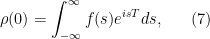
It is convenient, for the approach adopted here, to assume that the system is initialised in an eigenstate of ${T = \sum_{j} |j+1\rangle\langle j| + \mbox{h.c.}}$ . We write these eigenstates as

$\displaystyle |W(k)\rangle = \frac{1}{\sqrt{n}}\sum_{j=0}^{n-1} e^{\frac{2\pi i}{n} jk} |j\rangle. \ \ \ \ \ (3)$

We now develop an evolution equation for ${\rho(t)}$ in the interaction picture via the approach described in the previous post (i.e. via introduction of a fictitious ancilla ${R}$ system per site):

$\displaystyle \frac{d\rho(t)}{dt} = \int_0^t \mathcal{K}(\rho(s)) ds, \ \ \ \ \ (4)$

where ${\mathcal{K}(\cdot)}$ is the memory kernel. Carrying out the approximation described there yields

$\displaystyle \frac{d\rho_S(t)}{dt} = -\int_0^t dt_1 \mbox{tr}_R \left([V(t),[V(t_1),\rho_S(t)\otimes|G\rangle_R\langle G|]]\right) \ \ \ \ \ (5)$

where

$\displaystyle \begin{array}{rcl} |G\rangle &= \int \sqrt{p(\mathbf{x})}|\mathbf{x}\rangle d\mathbf{x}\\ &= \frac{1}{(\pi\mu)^{n/4}}\int e^{-\frac{\|\mathbf{x}\|^2}{2\mu}}|\mathbf{x}\rangle d\mathbf{x} \end{array}$

encodes the probability distribution for ${\mathbf{x}}$ . If we now trace out the fictitious ancillas we arrive at

$\displaystyle \frac{d\rho(t)}{dt} = -\frac{\mu}{2}\sum_{j=0}^{n-1}\int_0^t dt_1 [e^{-itT}|j\rangle\langle j|e^{itT},[e^{-it_1T}|j\rangle\langle j|e^{it_1T},\rho(t)]] \ \ \ \ \ (6)$

Writing out the commutators and carrying out the sum over ${j}$ gives:

$\displaystyle \begin{array}{rcl} \frac{d\rho(t)}{dt} =& \\ &-\frac{\mu}{2}\int_0^t dt_1 (\alpha(t-t_1) e^{-i(t-t_1)T}\rho(t) + \mbox{h.c.}) \\ &+\frac{\mu}{2}\int_0^t dt_1 (e^{-itT}\mbox{diag}(e^{itT}\rho(t)e^{-it_1T})e^{it_1T} + \mbox{h.c.}), \end{array}$

where ${\alpha(u) = \mbox{diag}(e^{iuT})}$ (which can be expressed in terms of a bessel function of the first kind, see the previous post). Notice a peculiarity of this evolution equation: if ${\rho(t)}$ is a function solely of ${T}$ at ${t=0}$ then it remains so for all time. Thus, eg., if we can write

$\displaystyle \rho(0) = \int_{-\infty}^{\infty} f(s) e^{isT} ds, \ \ \ \ \ (7)$

then we learn that for all ${t}$ we can always write

$\displaystyle \rho(t) = \int_{-\infty}^{\infty} f(s,t) e^{isT} ds, \ \ \ \ \ (8)$

Although the expansion (8) is not completely general, it will allow us to study the dynamics of the system initialised in an eigenstate of ${T}$ as there exist functions ${w_k(s)}$ such that

$\displaystyle |W(k)\rangle\langle W(k)| = \int_{-\infty}^{\infty} w_k(s) e^{isT} ds. \ \ \ \ \ (9)$

Let’s now go with the expansion (8) and try to derive an evolution equation for ${f(s,t)}$ :

$\displaystyle \begin{array}{rcl} \int_{-\infty}^{\infty} \frac{\partial f(s,t)}{\partial t} e^{isT} ds =& \\ -\frac{\mu}{2}\int_{-\infty}^{\infty}\int_0^t dt_1 (\alpha(t-t_1)f(s,t)e^{i(s-t+t_1)T} + \mbox{h.c.})ds \\ +\frac{\mu}{2}\int_{-\infty}^{\infty}\int_0^t dt_1 (\alpha(s+t-t_1)f(s,t) e^{-i(t-t_1)T} + \mbox{h.c.})ds. \end{array}$

A change of variable gives us

$\displaystyle \begin{array}{rcl} \int_{-\infty}^{\infty} \frac{\partial f(s,t)}{\partial t} e^{isT} ds =& \\ -\frac{\mu}{2}\int_{-\infty}^{\infty}\int_0^t du (\alpha(u)f(s+u,t) + \mbox{h.c.})du e^{isT}ds \\ +\frac{\mu}{2}\int_0^t \int_{-\infty}^{\infty} (\alpha(s+u)f(s,t) e^{-iuT} + \mbox{h.c.})ds du. \end{array}$

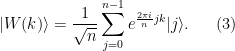
Defining

$\displaystyle \chi_{[0,t]}(u) = \begin{cases} 1, \quad0\le u\le t \\ 0, \quad\mbox{otherwise}\end{cases} \ \ \ \ \ (10)$

allows us to write

$\displaystyle \begin{array}{rcl} \int_{-\infty}^{\infty} \frac{\partial f(s,t)}{\partial t} e^{isT} ds =-\frac{\mu}{2}\int_{-\infty}^{\infty} g_1(s) e^{isT}ds +\frac{\mu}{2}\int_{-\infty}^{\infty} g_2(u,t) e^{iuT} du, \end{array}$

where

$\displaystyle g_1(s,t) = \int_0^t du (\alpha(u)f(s+u,t) + \mbox{h.c.})du \ \ \ \ \ (11)$

and

$\displaystyle g_2(u,t) = \chi_{[0,t]}(u)\int_{-\infty}^{\infty} (\alpha(s+u)f(s,t) + \mbox{h.c.})ds. \ \ \ \ \ (12)$

Thus we arrive at the following evolution equation for ${f(s,t)}$

$\displaystyle \begin{array}{rcl} \frac{\partial f(s,t)}{\partial t} =& \\ -\frac{\mu}{2}\int_0^t du (\alpha(u)f(s+u,t) + \mbox{h.c.})du \\ +\frac{\mu}{2}\chi_{[0,t]}(s)\int_{-\infty}^{\infty} (\alpha(s+u)f(u,t) + \mbox{h.c.})du. \end{array}$

Putting back in the hermitian conjugate terms leaves us with

$\displaystyle \begin{array}{rcl} \frac{\partial f(s,t)}{\partial t} =& \\ -\frac{\mu}{2}\int_{-t}^t \alpha(u)f(s+u,t) du\\ +\frac{\mu}{2}\chi_{[-t,t]}(s)\int_{-\infty}^{\infty} \alpha(u)f(s+u,t) du, \end{array}$

which can be rewritten as

$\displaystyle \begin{array}{rcl} \frac{\partial f(s,t)}{\partial t} =& \\ -\frac{\mu}{2}\int_{-\infty}^\infty (\chi_{[-t,t]}(u)-\chi_{[-t,t]}(s)) \alpha(u)f(s+u,t) du. \end{array}$

Such an equation can be expressed in terms of the convolution operation (in the ${s}$ variable) as

$\displaystyle \frac{\partial f(s,t)}{\partial t} = -\frac{\mu}{2} ((\alpha\chi_{[-t,t]})\star f) + \frac{\mu}{2} \chi_{[-t,t]}(s)(\alpha\star f). \ \ \ \ \ (13)$

This equation is amenable to solution via a fourier transform in ${s}$ and a laplace transform in ${t}$ . I’ll discuss it’s solution in another post.

This entry was posted on Tuesday, June 30th, 2009 at 11:11 am and is filed under disordered quantum systems. You can follow any responses to this entry through the RSS 2.0 feed. You can leave a response, or trackback from your own site.

Tobias J. Osborne's research notes